Within-stem maps of wood density and water content for characterization of species: a case study on three hardwood and two softwood species

Abstract

• Key message Variability and interrelations between wood density, water content, and related properties were analyzed by CT scanning of five species. Relative water content of lumens is proposed as the best complement to basic specific gravity for discrimination of species with respect to their functioning.

• Context X-ray computed tomography (CT) is an efficient tool for analysis of wood properties related to density and water content all along a tree stem. Basic specific gravity, an inherent property of the wood material, is well known and widely used in wood sciences.

• Aims The first aim of this study was to describe a method for mapping a set of wood properties within a tree stem. The second objective was to analyze the relations among these properties and to identify the one that offers the best information in addition to basic specific gravity for discrimination of species.

• Methods Wood discs were collected at various heights along a tree stem. We used a method consisting of comparing the CT images of the discs in the green state and after oven drying. Finally, 10 variables were computed for 115 trees of five temperate species: green, oven-dry, and basic specific gravities; moisture content; relative water content; relative water content of lumens; and fractions of air, water, free water, and cell walls.

• Results Maps of wood properties summarizing the radial and vertical variations were obtained, allowing us to highlight species-specific patterns. The five species were discriminated best when plotted in the plane defined by basic specific gravity and relative water content of lumens.

• Conclusion The proposed method is original and simple enough to process large samples. Because it correlated less with basic specific gravity than with moisture content, relative water content of lumens was selected for species characterization. This is the first study of such wood properties at this fine scale within a tree stem, simultaneously and for a substantial number of trees of five species including both hardwoods and softwoods.

1 Introduction

Numerous wood properties can be quantified for studies on tree growth, tree functioning, tree mechanical behavior, or wood quality. The sampling of increment cores or discs is the usual approach and enables researchers to retrospectively understand wood formation and to study wood properties and their variations.

X-ray computed tomography (CT) is a method that is widely used to measure wood density and is known to be accurate (Lindgren 1991; Freyburger et al. 2009; Watanabe et al. 2012). One of the advantages of CT scanning is that it provides detailed maps of density (CT slices), not only an average value for a sample. By measuring wood density of a given sample both at given moisture content and in the oven-dry state, it is possible to compute a large set of variables representing wood properties. For example, Fromm et al. (2001) illustrated the possibility to assess, through CT scanning, wood density, and water content by subtracting dry-density profiles from fresh-density profiles.

Some wood properties are inherent to the wood material, e.g., basic specific gravity (BSG). Other properties vary with time and are interesting in particular for studying living trees or when they are measured in green-wood samples, e.g., moisture content (MC) and relative water content (RWC).

Some properties and their variations are studied because they are related to the quality of the wood material (e.g., Ormarsson and Cown 2005; Forest Products Laboratory 2010), while others are studied because they provide information on some functional characteristics (Chave et al. 2009). BSG (or sometimes oven-dry or air-dry SG) is widely studied for several reasons: (1) it is a key variable of wood quality because it strongly correlates with physical and mechanical properties of dry clear wood, (2) it is useful for estimates of biomass and carbon stock and flux in studies on forest resources (Nogueira et al. 2008), and (3) although this topic is controversial (Larjavaara and Muller-Landau 2010; Zanne et al. 2010), BSG is also an indicator of some mechanical and hydraulic traits (Hacke et al. 2001; Chave et al. 2009). Green (or fresh) SG is interesting for explaining some mechanical characteristics related to standing trees. It is also important for logistical parameters of wood transportation after harvesting because it allows to calculate green weight from green volume. Wood MC and its distribution within stems is an input required for estimation of a biomass value per ton of fresh wood after harvesting and for control of subsequent drying or conversion-to-energy processes. The relative water content of lumens can be linked to hydraulic functioning because it provides information on the rate of lumen utilization for water transportation.

In this work, 10 variables were computed and studied: basic, oven-dry, and green-specific gravities; relative water content; the relative water content of lumens; moisture content; and volumetric fractions of cell walls, of total water, of free water, and of gas. Three hardwood species (Quercus petraea/robur, Fagus sylvatica, and Acer pseudoplatanus) and two softwood species (Abies alba and Pseudotsuga menziesii) were studied. The method that we developed in this work is based on X-ray analysis of discs in fresh and oven-dry states; this approach is original and gives access to three-dimensional (3D) within-stem variations of the above variables. Because it requires few manual interventions and no complex or time-consuming data processing, the method is fast enough to be applied to large sample sizes. Here, 1228 wood discs from 115 trees were processed; this sampling makes our work novel and original. The advantages and drawbacks of the method will be discussed and then two questions will be answered:

• Among the variables under study, which one is the most complementary to basic specific gravity for discrimination of species?

• What information about the functioning of our five temperate-zone tree species can be gained from this complementarity?

The species-specific patterns of radial and vertical variations within stems and a comparison with typical patterns from the literature will be the subject of a second paper.

2 Materials and methods

2.1 Experimental material

A total of 115 trees of five temperate species were sampled: three hardwood species (Q. petraea/robur, F. sylvatica, and A. pseudoplatanus) and two softwood species (A. alba and P. menziesii). The Quercus trees could be either Q. petraea or Q. robur because the two species were not differentiated in the field.

The Q. petraea/robur, F. sylvatica, and A. pseudoplatanus trees were sampled within the framework of the EMERGE project, which was aimed at the development of models for evaluation of the available forest biomass in France (Deleuze et al. 2010; Rivoire et al. 2010). The F. sylvatica and A. pseudoplatanus trees were sampled in February 2009 in a mixed even-aged high forest located in Montiers forest (48.538 N, 5.305 E). This means that this stand was managed as an even-aged high forest and had the appearance of an even-aged high forest. In this regional area and for these species, the regeneration periods are usually ∼30 years; this situation can explain the differences in age observed among the trees (Table 1). The Q. petraea/robur trees were sampled in February 2010 in a pure high forest located in Amance (48.764 N, 6.329 E). The A. alba and P. menziesii trees were sampled within the framework of the joint project Modelfor between INRA and ONF. The A. alba trees were sampled in April 2014 in two mixed even-aged high forests of A. alba and P. abies located in Mont-Sainte-Marie forest (46.789 N, 6.308 E) and in Saint-Prix forest (46.971 N, 4.069 E). The P. menziesii trees were sampled in March 2015 in a 20-year-old plantation in Quartier forest (46.149 N, 2.767 E) and in a 43-year-old plantation in Le Grison forest (46.662 N, 4.736 E).

Table 1 Characteristics of the sampled trees

All the trees were sampled in winter or at the beginning of spring before the trees start their annual growth; the purpose was to limit the possible effect of the transient nature of some moisture-related variables.

In each stand, dominant, codominant, and dominated trees were sampled so that the samples were representative of the resource.

The diameter at breast height (DBH), height of the first living branch for hardwood species, height of the first living whorl for softwood species, and total tree length were measured.

Wood discs were sampled along the stem: every 2 m from the ground for Q. petraea/robur, F. sylvatica, and A. pseudoplatanus; at the maximum, every 2 m for A. alba and P. menziesii. A radial cut was made using a band-saw on each disc to avoid drying checks. The radial cut was made at the same azimuthal position for all the discs of a given tree.

Table 1 shows characteristics of the sample trees.

2.2 CT scanning

The discs were scanned twice: (1) in the fresh state, after less than 1 week of storage in a plastic bag inside a cold room after harvesting and (2) in the oven-dry state, after 24 h of drying at 103 ^∘C and attainment of a stable weight. It is particularly important to dry the wood samples at temperatures above 100 ^∘C to remove all the water (including bound water). Williamson and Wiemann (2010) pointed out that in numerous recent studies, researchers made errors in measurements of wood-specific gravity (SG) by drying samples at temperatures ∼70 ^∘C.

At both stages, the discs from each tree were placed vertically and parallel to each other onto the scanner table, separated by a foam folder, and were all scanned together. Scanning was performed by means of an X-ray generator set to 80–120 kV and 50 mA for the fresh state and to 80 kV and 50 mA for the dry state. Slice thickness was set to 1.25 mm. The reconstruction was performed using the BONE filter¹ with a pixel size of 0.18 to 0.98 mm depending on the disc diameter.

2.3 Image processing

A set of ImageJ plug-ins and R (R Core Team 2014) scripts was used to process the images and average SG values in approximately the same areas for the fresh and dry states:

• A semiautomatic procedure was used to extract (from the stacks of images) the middle slice of each scanned disc. One CT slice per disc was analyzed in this study.

• The original DICOM images, in which grey levels are expressed in Hounsfield numbers, were converted into SG by applying the calibration described by Freyburger et al. (2009).

• The disc contour at the wood–bark boundary, the pith location, and the opening angle and azimuth of the radial split were recorded manually on the images for the fresh and dry states.

• Cubic spline interpolation was used to model the distance to the pith of the disc contour as a function of the azimuth. For each pixel of the image, the distance to the pith r and the angle from the split beginning a were computed (Fig. 1). These data were used to calculate relative polar coordinates for each pixel, i.e., the relative radius, as the ratio of r to the disc radius R, and relative azimuth, as the ratio of a to the disc’s opening angle A=2π−𝜃, where 𝜃 is the split opening angle. Both the relative radius and azimuth varied in the range 0 to 1 regardless of the image, making it possible to compare the discs in the fresh and dry states.

  Fig. 1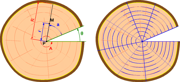

  

  The sectorization method: the relative polar coordinates of pixel M are obtained from the ratios r/R and a/A varying in the range 0 to 1; the discs are then divided into 1-cm-thick tangential bands and a certain number of angular sectors

  The discs were divided into tangential bands of fixed mean width (equal to 1 cm in the fresh state), the remaining area near the pith being larger than 1 cm to complete the radius. The contours of the tangential bands were obtained by homothety of the external contour. In the dry state, the mean band width was set to 1 cm multiplied by the ratio of the mean radius in the dry state divided by the mean radius in the fresh state. The pixels belonging to each band were counted and averaged, giving the area and mean SG in the fresh (green) and dry states. Only the pixels with SG ranging from 0.2 to 1.4 were considered in order to eliminate drying checks and possible inclusions of nonwood materials.

  By computing the mean values of the bands, we could analyze the radial variations of SG in the fresh and dry states. It would have been possible to analyze the tangential variations as well by dividing the bands into angular sectors (Fig. 1), but this option was not used in the present study.

2.4 Computation of the variables

From the raw data described above, green SG (S G _g ), oven-dry SG (S G ₀), basic SG (BSG), moisture content (MC), relative water content (RWC), relative water content of lumens (R W C _L ), and volumetric fractions of cell walls, of total water, of free water, and of gas were calculated for each band.

Green SG and oven-dry SG were obtained directly from the averaged pixel values (Section 2.3). Other variables were computed as follows:

$$ BSG = \frac{W_{0}} {V_{g}} \cdot \frac{1}{\rho_{\text{water}}} = SG_{0} \cdot \frac{V_{0}} {V_{g}} \approx SG_{0} \cdot \frac{S_{0}} {S_{g}} $$

(1)

$$ MC = \frac{W_{g} - W_{0}} {W_{0}} \cdot 100 \approx \frac {SG_{g} \cdot S_{g} - SG_{0} \cdot S_{0}} {SG_{0} \cdot S_{0}} \cdot 100 \\ $$

(2)

where V _g and V ₀ are the volumes in the green and dry state, respectively, W _g and W ₀ are the corresponding weights, S G _g and S G ₀ are the corresponding values of measured average SG, S _g and S ₀ are the measured areas, and ρ _water is the density of water. We assumed here that moisture content in the green state was always above the fiber saturation point (FSP).

The relative water content (RWC) is the ratio of the amount of water in the sample to the amount of water at full saturation. RWC varies from 0 in the oven-dry state to 100 at saturation. RWC in the green state was computed assuming constant cell wall density ρ _walls by means of the following formula derived from the work of Bouffier et al. (2003):

$$\begin{array}{@{}rcl@{}} RWC &=& \frac{W_{\text{water, g}}} {W_{\text{water, sat}}} = \frac{W_{g} - W_{0}} {(V_{g} - W_{0}/\rho_{\text{walls}}) \cdot \rho_{\text{water}}} \cdot 100\\ &=& \frac{SG_{g} - BSG} {1 - BSG \cdot \frac{\rho_{\text{water}}} {\rho_{\text{walls}}}} \cdot 100 \end{array} $$

(3)

where ρ _water is the density of water and ρ _walls the density of wood cell walls. We assumed here that $\rho _{\text {water}} = 1000~\text {kg}~\text {m}^{-3}$ and $\rho _{\text {walls}} = 1500~\text {kg}~ \text {m}^{-3}$.

Another definition of the relative water content has been proposed to better reflect the water content of lumens. The relative water content of lumens (R W C _L ) can be computed by subtracting the weight of water contained within the sample at FSP, corresponding to the amount of water in cell walls above FSP, from both the numerator and the denominator of the original RWC. Hence, bound water is removed, and R W C _L should better reflect the level of lumen utilization and may probably be a better representation of hydraulic functioning.

$$ RWC_{L} = \frac{W_{\text{water, g}} - W_{\text{water, FSP}}} {W_{\text{water, sat}} - W_{\text{water, FSP}}} \cdot 100 = \frac{SG_{g} -K}{SG_{sat} - K} \cdot 100 $$

(4)

with:

$$K = \left( 1 + \frac{MC_{FSP}}{100}\right) \cdot BSG $$

where W _{water, g}, W _{water, FSP}, and W _{water, sat} are, respectively, the weight of water in the green state, at the fiber saturation point, and at full saturation. M C _{F S P} is the moisture content at the fiber saturation point, which was assumed to be 30 % (Forest Products Laboratory 2010). S G _{s a t} is the SG at full saturation, which can be computed as

$$\begin{array}{@{}rcl@{}} SG_{sat} &=&\frac {W_{0} + W_{\text{water, sat}}}{V_{g} \cdot \rho_{\text{water}}} = 1 + BSG \cdot \left( 1 - \frac{\rho_{\text{water}}}{\rho_{\text{walls}}} \right) \\ &&\approx 1 + \frac{BSG}{3} \end{array} $$

(5)

Finally, the volumetric fractions of water (f _water), of free water ($f_{\text {free\_water}}$), of gas (f _gas), and of cell walls (f _walls) in green wood were calculated via the following equations:

$$ f_{\text{walls}} = \frac{V_{\text{walls}}} {V_{g}} = BSG \cdot \frac{\rho_{\text{water}}}{\rho_{\text{walls}}} \approx \frac{2}{3} \cdot BSG $$

(6)

$$ f_{\text{water}} = \frac{V_{\text{water}}} {V_{g}} = SG_{g} - BSG = \frac {MC \cdot BSG} {100} $$

(7)

The fraction of free water was computed by removing the fraction of bound water (mathematically related to BSG) from the fraction of total water:

$$ f_{\text{free\_water}} = \frac{V_{\text{free\_water}}} {V_{g}} = f_{\text{water}} - \frac{MC_{\text{FSP}} \cdot BSG}{100} $$

(8)

The fraction of gas was computed as

$$ f_{\text{gas}} = \frac{V_{\text{gas}}} {V_{g}} = 1 - f_{\text{water}} - f_{\text{walls}} $$

(9)

and may also be expressed as

$$ f_{\text{gas}} = \left( 1-\frac{RWC_{L}}{100}\right) \cdot \left( 1 - BSG \cdot \left( \frac{\rho_{\text{water}}} {\rho_{\text{walls}}} + \frac{MC_{\text{FSP}}}{100}\right)\right) $$

(10)

In the above equations, V _walls, V _water, $V_{\text {free\_water}}$, and V _gas are the volumes of cell walls, of total water, of free water, and of gas in the green volume V _g .

2.5 Statistical analysis

We used the statistical software package R (R Core Team 2014).

To calculate the disc averages, the surfaces and weights of the tangential bands were summed and substituted into Eqs. 1 to 9. The tree averages were calculated in the same way by summing the volumes and weights of truncated cones centered on each disc.

The akima R package was used for bilinear interpolation of the data and to build 2D maps of the wood properties illustrating variations in both the radial direction and vertical direction.

3 Results

3.1 Relations among the computed variables

Figure 2 shows a matrix of plots for the set of computed variables illustrating both intraspecies (at the disc level) and interspecies relations. The upper part of the matrix shows Pearson’s correlation coefficients per species.

Fig. 2

Relations among the variables green-specific gravity (S G _g ), basic specific gravity (BSG), moisture content (MC), relative water content of lumens (R W C _L ), free water fraction ($f_{\text {free\_water}}$) and gas fraction (f _gas). Each point represents a disc sample. The upper right-hand panels show Pearson’s correlation coefficients and p values by species (*** <0.001, ** <0.01, * <0.05)

The variable f _walls is not presented in Fig. 2 because it is mathematically proportional to BSG (Eq. 6). When a positive correlation between two variables was too strong, only one of them was retained in the plot. This was the case for the pairs of variables S G ₀ with BSG, RWC with R W C _L , and f _water with $f_{\text {free\_water}}$ (Fig. 3).

Fig. 3

Relations among strongly correlating variables: oven-dry specific gravity (S G ₀) and basic specific gravity (BSG), relative water content (RWC) and relative water content of lumens (R W C _L ), water fraction (f _water), and free water fraction ($f_{\text {free\_water}}$). Each point represents a disc sample

The slope of the relation between BSG and S G ₀ depends mathematically on S ₀/S _g (Eq. 1), which strongly correlates with 1−s h r i n k a g e. This means that the slope of the relation is closest to 1 for the smallest shrinkage values; this situation is consistent with the observed value of a slope close to 1 for the softwood species and lower for the hardwood species, especially for F. sylvatica and Q. petraea/robur (Fig. 3). Finally, we decided to use BSG instead of S G ₀ in further analyses because the former is a more widely used variable in our field of wood research.

R W C _L and RWC also correlated strongly (Eqs. 3 and 4), with a deviation from the y=x line greater for the hardwood species than for the softwood species (Fig. 3). This result means that the softwood species contain proportionally less bound water (in comparison with free water) than do the hardwood species that have higher wood density. We decided to keep R W C _L instead of RWC, because above FSP, the variations in water content are related to free water content only, and because it enabled a better understanding of some physiological characteristics related to lumen utilization for conduction.

Variables f _water and $f_{\text {free\_water}}$ correlated strongly, with a slope close to 1 regardless of the species and with the intercept depending on the wood density of the species (Fig. 3). We decided to keep $f_{\text {free\_water}}$ instead of f _water for the same reasons we kept R W C _L instead of RWC.

S G _g strongly negatively correlated with the volumetric fraction of gas (f _gas), i.e., strongly positively correlated with the cumulated fraction of cell walls and water, independently of the proportions of cell walls and water. S G _g strongly positively correlated with R W C _L at the intraspecies level. At the interspecies level, the points for softwoods shifted toward higher values of R W C _L in comparison with hardwoods for equivalent values of S G _g . This observation means that variations in green SG can be explained mostly by variations in water content (variables R W C _L and $f_{\text {free\_water}}$), water content being an important source of heterogeneity within the stems of trees for a given species and among species. To a lesser extent, green SG was also dependent on BSG, mainly for hardwoods.

MC negatively correlated with basic SG both at intra- and interspecies levels and positively correlated with $f_{\text {free\_water}}$ and with R W C _L , mostly at the intraspecies level for the latter. For example, F. sylvatica had high R W C _L but quite low MC because of dense wood (high BSG), whereas A. alba had high R W C _L associated with wood of lower density, which resulted in high MC.

Regardless of the species, BSG was relatively independent of R W C _L and f _gas. Both variables could therefore be considered a useful complement of BSG for species characterization and discrimination.

A strong negative correlation was observed between the fraction of gas (f _gas) and water saturation of lumens (R W C _L ), with a slope depending on the species.

The relation between BSG and R W C _L was plotted at tree, disc, and tangential band levels (Fig. 4). The results were similar at the tree and disc levels (with slightly greater variations at the disc level than at the tree level). This finding means that the vertical variations within stems were rather low. The variations were much greater at the tangential band level, especially in terms of the water content variable R W C _L , which indicates substantial radial variation within discs.

Fig. 4

Relations between the relative water content of lumens (R W C _L ) and basic specific gravity (BSG) at three levels of variabilit

3.2 Within-stem variations by species

For illustration of possible output of our method, some maps of within-stem variations for each species are presented in Figs. 5 and 6. The full set of maps for BSG, R W C _L , MC, green SG, the free water fraction, and air fraction is available as Online Resources (Appendices A to F). The radial and vertical variations and their differences among the species will be analyzed in more detail in the second paper.

Fig. 5

Maps of basic specific gravity (BSG) and the relative water content of lumens (R W C _L ) for three hardwood trees (Fagus #92, Acer #80, Quercus #1005)

Fig. 6

Maps of basic specific gravity (BSG) and the relative water content of lumens (R W C _L ) for two softwood trees (Abies #PW4 and Pseudotsuga #GT3)

3.2.1 Fagus sylvatica

Most of the F. sylvatica trees showed higher BSG at the bottom and at the top of the stem, i.e., a U-shape profile of BSG. The trees often showed wood of lower density within a small area located around the pith. MC and R W C _L were higher in the external part of the stem, with a drier and less saturated area around the pith. Hence, F. sylvatica showed a limited corewood area, less dense and drier than the outer wood, while wet and highly saturated areas covered a substantial part of the stems in this species.

3.2.2 Acer pseudoplatanus

Overall, A. pseudoplatanus (just as F. sylvatica) showed higher BSG both at the bottom and at the top of the stem and lower BSG at midheight near the pith. BSG and the water-related variables (green SG, MC, R W C _L , and $f_{free\_water}$) increased radially. The wet and highly saturated areas were located near the pith at the bottom of some stems and in the most external part of the stem (a more restricted area than in F. sylvatica).

3.2.3 Quercus petraea/robur

In contrast to F. sylvatica and A. pseudoplatanus, Q. petraea/robur showed a radial decrease in BSG, with a lower density band parallel to the bark. Areas of higher MC and R W C _L were observed in the most external part of the stem as a rather narrow band parallel to the bark and around the pith in the lower part of the stems.

3.2.4 Abies alba

BSG was relatively constant radially. Greater BSG was often observed at the bottom of the stem in this species. Strong radial variation of the water-related variables was clearly visible on the maps. In addition, some trees showed wet corewood at the bottom of the stem near the pith.

3.2.5 Pseudotsuga menziesii

P. menziesii showed higher BSG at the bottom of the stem, just as A. alba did, but in contrast to A. alba, an obvious radial increase in BSG was observed in almost all the trees. The water-related variables showed even stronger contrast than in A. alba between dry inner wood (MC often below 50 %) and wet outer wood (MC above 100 %). No wet corewood was observed in this species.

3.3 Interspecies variations

Table 2 shows means and standard deviations of the variables. The computations were performed on the basis of whole-stem measurements (as weighted means of discs at several heights).

Table 2 Means and standard deviations of the computed variables by species: green specific gravity (S G _g ), oven-dry specific gravity (S G ₀), basic specific gravity (BSG), moisture content (MC), relative water content (RWC), relative water content of lumens (R W C _L ), water fraction (f _water), gas fraction (f _gas), walls fraction (f _walls), and free water fraction ($f_{\text {free\_water}}$)

BSG was the greatest in F. sylvatica (0.59) and in Q. petraea/robur (0.58). A. pseudoplatanus, P. menziesii, and A. alba showed lower values: 0.49, 0.42, and 0.35, respectively.

MC values were equal for F. sylvatica and A. pseudoplatanus (87 %) but somewhat lower for Q. petraea/robur (74 %), somewhat higher for P. menziesii (104 %), and more than twice higher for A. alba (193 %).

On the other hand, regarding the relative water content of lumens (R W C _L ), A. alba and F. sylvatica showed the highest values, 86 and 80 %, respectively, whereas A. pseudoplatanus, Q. petraea/robur, and P. menziesii showed lower values (54, 58, and 52 %, respectively).

In terms of the fractions of cell walls, water, and gas (Fig. 7), the five species showed contrasting patterns: F. sylvatica and Q. petraea/robur had the same proportion of cell walls (∼40 %) but were different in terms of water and air fractions; A. pseudoplatanus and Q. petraea/robur had the same proportion of water (43 %) but differed in fractions of wood cell walls and air; F. sylvatica and A. alba had the same proportion of air (9 %) but differed in fractions of cell walls and water. On average, P. menziesii and A. pseudoplatanus had almost the same proportions of cell walls, water, and gas.

Fig. 7

Average fractions of cell walls (orange), of water (blue), and of gas (sky blue) observed in each species

4 Discussion

4.1 Advantages and drawbacks of the method

CT scanning is a reliable and accurate method for measurement of wood density regardless of tree species and scanner settings (Lindgren 1991; Freyburger et al. 2009). Today, the price of medical scanners is reasonable, and it is even possible to buy second-hand scanners from hospitals. Many wood research labs now have access to such equipment for studies on internal wood structure and properties.

Our method is based on processing of CT images of wood discs and enables creation of maps of oven-dry and green SG at high radial and tangential resolution. In this study, good integration of local tangential variations was obtained via calculation of variables within tangential bands, each band corresponding more or less to a group of successive annual rings. The longitudinal resolution depended on the number of discs considered along the stems.

In particular, one advantage of the proposed method is that measurements are done on whole discs, without overestimation of the volume of corewood and heartwood and with consideration of all azimuthal positions, contrary to measurements based on wood increment cores (Williamson and Wiemann 2010; Osazuwa-Peters et al. 2014).

The method allows us to compare CT images of discs in fresh and oven-dry states and thus to compute basic SG and MC, which are not directly accessible via CT scans. Here, we implicitly assumed that shrinkage due to the moisture change is negligible in the longitudinal direction and homogeneous in the transverse directions (but not assuming equal shrinkages in radial and tangential directions). The latter assumption is a nontrivial hypothesis because both radial and tangential shrinkage values are known to depend on wood properties (e.g., Gryc et al. 2008, for beech). Nevertheless, we assumed that the field of deformation was regular enough to allow for comparison of “reasonably” large regions. The advantage is that the method is easy to implement and perfectly suitable for processing of wood disc images. This is not the case for other (more complex) approaches proposed in the literature (e.g., Lindgren 1992; Watanabe et al. 2012).

For comparison, the BSG values from the Global Wood Density Database (Zanne et al. 2009) are 0.585, 0.509, 0.560, 0.353, and 0.453 for F. sylvatica, A. pseudoplatanus, Q. petraea/robur, A. alba, and P. menziesii, respectively. Our measurement data are consistent with these values, with slightly greater BSG for F. sylvatica than for Q. petraea/robur.

Then, under the assumption of constant density of cell walls ($\rho _{walls} = 1500~\text {kg}~\text {m}^{-3}$), the method enables us to estimate RWC and water, gas, and cell wall fractions in the fresh state (i.e., as in a living tree in the present study). The value of 1500 kg m⁻³ is widely accepted in the fields of tree growth and wood quality. It is known, however, that ρ _walls density depends on species, sample preparation, and the method of measurement (Zauer et al. 2013). Stamm (1929) obtained values for ρ _walls between 1484 and 1536 kg m⁻³. Kellogg and Wangaard (1969) after analyzing 18 species found that ρ _walls values range from 1497 to 1517 kg m⁻³ for the hardwoods and from 1517 to 1529 kg m⁻³ for the softwoods studied. This result contradicts the findings of Zauer et al. (2013) who observed lower cell wall density in softwood than in hardwood. In a recent study, Plötze and Niemz (2011) obtained an average value of 1493 kg m⁻³ with a minimum of 1458 kg m ⁻³ for Nauclea diderrichii and a maximum of 1528 kg m⁻³ for Q. robur. The value for F. sylvatica is 1472 kg m⁻³. Zauer et al. (2013) reported the value of 1510 kg m⁻³ for A. pseudoplatanus. On the basis of this review of the literature and in the absence of a large study on temperate species reporting density data on wood cell walls for the five species analyzed here, a common ρ _walls value of 1500 kg m⁻³ is the best choice.

Finally, if we assume MC of 30 % at the fiber saturation point, the method allows to estimate the relative water content of lumens (R W C _L ). The value of 30 % is widely accepted in the community of wood researchers (Forest Products Laboratory 2010). Actually, M C _{F S P} varies depending on species (with smaller variation for temperate species than for tropical ones) and depending on the methods used to measure it (Babiak and Kúdela 1995). Unfortunately, there is no recent study providing these data on our five species by means of a common method of measurement (Zauer et al. 2014; Babiak and Kúdela 1995). Thus, the value of 30 % seems to be the best choice.

4.2 Which variables are the most suitable for discrimination of tree species?

All the studied variables are related to each other via physical relations (see Section 2) resulting from the concept of wood structure as a cellular solid. Nonetheless, the strength of a correlation between two variables depended on the variability of possible other variables also involved in the relation.

For characterization of the wood material, basic SG and MC are widely used variables. In this study, they strongly correlated negatively and thus yielded mainly the same information. This negative correlation was also reported by Nogueira et al. (2008) for tropical tree species.

Although MC is a well-known variable for characterization of wood moisture, below or above FSP (M C∼30 %), in air-dried wood (M C∼12 %), this variable was not suitable for characterization of traits related to species functioning. Indeed, MC does not provide clear information about the amount of water in green samples or in living trees. For example, F. sylvatica and A. pseudoplatanus showed similar MC, but F. sylvatica contained more water than did A. pseudoplatanus per unit of volume.

A particularly interesting result of our study is the absence of relation between basic SG and the relative water content of lumens (R W C _L ). Due to the relations among variables, a similar pattern was observed between the cell wall fraction (proportional to BSG) and gas fraction (negatively correlated with R W C _L ); these results seem to contradict those of Schüller et al. (2013) on tropical tree species. Among 27 tree species from the Mexican rain forest, they found no correlations at the interspecies level between water and cell wall fractions but a negative correlation between gas and cell wall fractions. This discrepancy between the two studies is apparently mainly due to the presence of the softwood species (A. alba and P. menziesii) in our study. Although less studied than water content, gas content may play mechanical and physiological roles in living trees. For example, Gartner et al. (2004) analyzed how the gas fraction in stems may affect the mechanical behavior of tree stems. The gas fraction affects the fresh mass of trees and is related to the stem growth in diameter because a large gas fraction ensures inexpensive growth of the stem without biomass investment. According to the review by Gartner et al. (2004), rather large gas fractions were reported for North American hardwood species both in sapwood and heartwood (26 % on average), whereas for North American softwood species, the reported gas fractions are 50 % and 18 % for heartwood and sapwood, respectively.

We found a negative correlation between the fractions of gas and water, but this relation was mostly observed at the intraspecies level and may be explained by a cell wall fraction that is relatively homogeneous for a given species. Actually, for given wood density, the more water there is, the less gas is present, and vice versa. At the interspecies level, in the presence of high variability in BSG (and cell wall fraction), the negative correlation between gas and water fractions is not necessarily guaranteed and was not observed in our study. Nonetheless, Schüller et al. (2013) observed such a negative correlation in their 27 tropical species.

Finally, water or gas fractions (in volume) or water saturation of wood (RWC or R W C _L ) yielded information that is much more complementary to BSG than MC and thus appear to be better choices for characterization of some species-specific traits mainly related to hydraulic functioning.

Several authors cited by Gartner et al. (2004) reported that the water fraction of wood in living trees of temperate zones shows seasonal variation, with a decrease from early spring to midsummer, then an increase until early winter. Our field measurements were performed at the very end of winter for all species, and water content may therefore be close to the maximum of the year. This assumption seems consistent with the review of the literature by Gartner et al. (2004) showing slightly lower water fractions for North American species (the dates of the measurements were not reported) than for our temperate species (41 % on average for hardwood species, 24 % for heartwood of softwood species, and 57 % for sapwood of softwood species).

Another source of MC variation in living trees is the process of heartwood formation, which depends on the species, tree age, stand management, tree vitality, and tree health (Longuetaud et al. 2006). In particular, softwood species have in general contrasting heartwood and sapwood (Lüttschwager and Remus 2007); this is not necessarily the case for hardwoods. For example, F. sylvatica does not show clear-cut delimitation between heartwood and sapwood, but rather a gradual transition (Gebauer et al. 2008). For Q. petraea/robur, the sapwood area as defined by its light color does not match the conductive sapwood and is not necessarily related to any difference in MC. Our sampling ensured a wide range of sapwood proportions because we chose contrasting species, including both hardwoods and softwoods, and contrasting stand management.

All trees belonged to the same age class (except Q. petraea/robur trees that were older and to a lesser extent, P. menziesii trees that were younger) and were sampled in winter in order to limit possible effects of water content variations with time. Despite the transient nature of the water-related variables, water content is known to be a suitable trait for physiological characterization of species. For example, early-successional genera such as Alnus, Populus, and Betula, and the sapwood of softwood species such as A. alba and P. menziesii in this study, are known to have relatively high water content in living trees.

4.3 What information about species functioning can be gained?

Overall, the highest-density woods (hardwoods) were characterized by the lowest MC both at intra- and interspecies levels. Hardwoods, with potentially smaller available space for free water than in softwoods, showed lower water fractions. This finding means that they contained less water per unit of volume than low-density woods did. On the other hand, if we consider hardwoods only, F. sylvatica, which had higher BSG than Q. petraea/robur did, at the same time showed a greater fraction of water and higher relative water content of lumens. More generally, the absence of a clear relation between BSG and R W C _L means that even if there was space for free water, this space was not necessarily filled with water. In particular, high-density woods were not necessarily more saturated with water than low-density woods did. In other words, high-density woods did not have to be filled with water to fulfill the water requirements of trees. Our result is concordant with the observations made by Gartner et al. (2004) on North American temperate species. Those authors concluded that whether cell lumens will be filled with water or gas is not determined by wood basic SG.

R W C _L and $f_{\text {free\_water}}$ appear to be interesting traits for characterization of hydraulic tree functioning because these variables are associated with the capacitance function of the species. A comparison (Appendix G) with the drought tolerance scores provided by Niinemets and Valladares (2006) showed that among our five temperate species of trees, the two with the greatest R W C _L and $f_{\text {free\_water}}$ (F. sylvatica and A. alba) are late-successional species and are the less drought tolerant. Conversely, Q. petraea/robur was found to be the most drought tolerant and at the same time showed the lowest fraction of free water.

5 Conclusion

A method for mapping of wood properties within tree stems on the basis of CT scans of wood discs is presented. This method is original and relatively easy to use; for this reason, it is suitable for large sample sizes. Scans of discs at two levels of moisture content are needed, including one scan in the oven-dry state. Ten variables were computed including wood density and water-related variables. Some of these variables are particularly original and have never been studied at this scale, for instance, the relative water content of lumens and the volumetric fraction of free water.

The relations among the variables were analyzed. Basic specific gravity and the relative water content of lumens (or the fraction of gas) were found to be relatively complementary. Thus, these variables are suitable for species characterization and discrimination.

According to our results, A. alba, F. sylvatica, and A. pseudoplatanus have contrasting characteristics, whereas Q. petraea/robur is somewhere between F. sylvatica and A. pseudoplatanus. P. menziesii was found to be a rather intermediate species between A. alba and the hardwood species. The species with the highest water saturation in their lumens and the greatest volumetric fraction of free water (A. alba and F. sylvatica) are also known to be less drought tolerant.

Our second paper will be focused on the species-specific patterns of radial and vertical variations of basic specific gravity and relative water content of lumens. A comparison with typical patterns of variations reported in the literature will also be conducted.

References

Babiak M, Kúdela J (1995) A contribution to the definition of the fiber saturation point. Wood Sci Technol 29:217–226
Bouffier L, Gartner B, Domec J-C (2003) Wood density and hydraulic properties of ponderosa pine from the Willamette valley vs. the Cascade mountains. Wood Fiber Sci 35:217–233
Chave J, Coomes D, Jansen S, Lewis S L, Swenson N G, Zanne A E (2009) Towards a worldwide wood economics spectrum. Ecol Lett 12:351–366
Deleuze C, Piboule A, Tricot E, Constant T, Longuetaud F, Mendow N, Rivoire M, Dassot M, Saint-André L, Genet A, Wernsdörfer H, Vallet P, Morneau F, Colin A, Bouvet A, Thivolle-cazat A, Gauhthier A, Jaeger M, Borianne P (2010) Reliable estimation of biomass in our forests? In: 18th European biomass conference and exhibition, Lyon, France, 3–7 mai, pp 61–66
Forest Products Laboratory (2010) Wood handbook: wood as an engineering material. General Technical Report FPL-GTR-190. USDA Forest Service Forest Products Laboratory, Madison
Freyburger C, Longuetaud F, Mothe F, Constant T, Leban J-M, DEC (2009) Measuring wood density by means of x-ray computer tomography. Ann For Sci 66:804
Fromm J H, Sautter I, Matthies D, Kremer J, Schumacher P, Ganter C (2001) Xylem water content and wood density in spruce and oak trees detected by high-resolution computed tomography. Plant Physiol 127:416–425
Gartner BL, Moore JR, Gardiner BA (2004) Gas in stems: abundance and potential consequences for tree biomechanics. Tree Physiol 24:1239–1250
Gebauer T, Horna V, Leuschner C (2008) Variability in radial sap flux density patterns and sapwood area among seven co-occurring temperate broad-leaved tree species. Tree Physiol 28 :1821–1830
Gryc V, Vavrcik H, Gomola S (2008) Selected properties of European beech (Fagus sylvatica L.). J For Sci 54:418–425
Hacke U G, Sperry J S, Pockman W T, Davis S D, McCulloh K A (2001) Trends in wood density and structure are linked to prevention of xylem implosion by negative pressure. Oecologia 126:457– 461
Kellogg RM, Wangaard FF (1969) Variation in the cell-wall density of wood. Wood Fiber Sci 1:180–204
Larjavaara M, Muller-Landau HC (2010) Rethinking the value of high wood density. Funct Ecol 24:701–705
Lindgren L (1991) Medical cat-scanning: X-ray absorption coefficients, ct-numbers and their relation to wood density. Wood Sci Technol 25:341–349
Lindgren O (1992) Medical ct-scanners for non-destructive wood density and moisture content measurements. Ph.D. thesis, Luleå Tekniska Universitet
Longuetaud F, Mothe F, Leban J-M, Mäkelä A (2006) Picea abies sapwood width: variations within and between trees. Scand J For Res 21:41–53
Lüttschwager D, Remus R (2007) Radial distribution of sap flux density in trunks of a mature beech stand. Ann For Sci 64:431–438
Niinemets Ü, Valladares F (2006) Tolerance to shade, drought, and waterlogging of temperate northern hemisphere trees and shrubs. Ecol Monogr 76:521–547
Nogueira E M, Fearnside P M, Nelson B W, Barbosa R I, Keizer E W H (2008) Estimates of forest biomass in the brazilian amazon: new allometric equations and adjustments to biomass from wood-volume inventories. For Ecol Manag 256:1853– 1867
Ormarsson S, Cown D (2005) Moisture-related distortion of timber boards of radiata pine: comparison with norway spruce. Wood Fiber Sci 37:424–436
Osazuwa-Peters OL, Wright SJ, Zanne AE (2014) Radial variation in wood specific gravity of tropical tree species differing in growth–mortality strategies. Am J Bot 101:803–811
Plötze M, Niemz P (2011) Porosity and pore size distribution of different wood types as determined by mercury intrusion porosimetry. Eur J Wood Wood Prod 69:649–657
R Core Team (2014) R: a language and environment for statistical computing. R Foundation for Statistical Computing, Austria. http://www.R-project.org/
Rivoire M, Deleuze C, Longuetaud F, Saint-André L, Morneau F, Vallet P, Bouvet A, Gauthier A (2010) Exploring the variability of biomass distribution in individual forest trees. In: XXIII IUFRO World Congress, Seoul
Schüller E, Martínez-Ramos M, Hietz P (2013) Radial gradients in wood specific gravity, water and gas content in trees of a mexican tropical rain forest. Biotropica 45:280–287
Stamm AJ (1929) Density of wood substance, adsorption by wood, and permeability of wood. J Phys Chem 33:398–414
Watanabe K, Lazarescu C, Shida S, Avramidis S (2012) A novel method of measuring moisture content distribution in timber during drying using ct scanning and image processing techniques. Dry Technol 30:256–262
Williamson GB, Wiemann MC (2010) Measuring wood specific gravity... correctly. Am J Bot 97:519–524
Zanne A, Lopez-Gonzalez G, Coomes D, Ilic J, Jansen S, Lewis S, Miller R, Swenson N, Wiemann M, Chave J (2009) Data from: towards a worldwide wood economics spectrum. doi:http://dx.doi.org/10.5061/dryad.234
Zanne AE, Westoby M, Falster DS, Ackerly DD, Loarie SR, Arnold SE, Coomes DA (2010) Angiosperm wood structure: global patterns in vessel anatomy and their relation to wood density and potential conductivity. Am J Bot 97:207–215
Zauer M, Pfriem A, Wagenführ A (2013) Toward improved understanding of the cell-wall density and porosity of wood determined by gas pycnometry. Wood Sci Technol 47 :1197–1211
Zauer M, Kretzschmar J, Großmann L, Pfriem A, Wagenführ A (2014) Analysis of the pore-size distribution and fiber saturation point of native and thermally modified wood using differential scanning calorimetry. Wood Sci Technol 48:177–193
Acknowledgments
Thanks to all the people who were involved in this project, especially all the people who contributed to field measurements. Special thank to Charline Freyburger and Pierre Gelhaye who helped with CT scanning and image processing.
Author information
Authors and Affiliations
Corresponding author
Ethics declarations
Funding
We would like to thank the French National Research Agency (ANR) that funded the research project EMERGE through its Bioenergy program.
A part of the data used in this work was collected within the frame of the Modelfor 2012–2015 joint project between INRA and ONF. The UMR 1092 LERFoB is supported by a grant overseen by the French National Research Agency (ANR) as part of the Investissements d’Avenir program (ANR-11-LABX-0002-01, Lab of Excellence ARBRE).
Additional information
Handling Editor: Jean-Michel Leban
Contribution of the co-authors
Fleur Longuetaud designed the experiment, run the data analysis and was the main writer. Frédéric Mothe designed the experiment, run the data analysis and contributed to the writing. Meriem Fournier contributed to the discussions and to the writing. Jana Dlouha contributed to the discussions and to the writing. Philippe Santenoise helped to run the data analysis and contributed to the writing. Christine Deleuze supervised the work, coordinated the EMERGE project and contributed to the writing.
This article is part of the Topical Collection on Estimation of standing forest biomass
Electronic supplementary material
Below is the link to the electronic supplementary material.
Rights and permissions
About this article
Cite this article
Longuetaud, F., Mothe, F., Fournier, M. et al. Within-stem maps of wood density and water content for characterization of species: a case study on three hardwood and two softwood species. Annals of Forest Science 73, 601–614 (2016). https://doi.org/10.1007/s13595-016-0555-4
Received:
Accepted:
Published:
Issue Date:
DOI: https://doi.org/10.1007/s13595-016-0555-4